GreyTheory

English | 繁體中文 | 日本語

Grey forecasting, feature comparison, and PCA for Python.

Documentation · Getting started · Workbench · Benchmarks

Forecast a short sequence, rank features against a target, or explore spectra and process measurements. Start with a few lines of Python, or use the bundled HTML workbench.

What you can do

• Combine Grey + PCA: GreyPCA brings six PCA backends together with GRA component selection. PCA summarizes sample differences; with a reference target, GRA scores and selects related components. For spectra, images, and paths, add Grey-window features before PCA to include local patterns.
• Forecast: GM11 and two-level Convolution; GM0N / GM1N for ordered multivariate data.
• Compare: GRA feature ranking and mixed larger / smaller / target quality preferences.
• Explore: six PCA backends, raw-count PoissonPCA, Grey windows, images, and multidimensional paths.

Quick start

Requires Python 3.11+. Download or clone the repository, then run:

python3 run.py

Tip

The first run prepares .venv and installs dependencies. On Windows, use python in place of python3.

Use the library

Install into the Python environment used by your own program:

python -m pip install .

from greytheory import GM11

series = [223.3, 227.3, 230.5, 238.1, 242.9, 251.1]
model = GM11(background_mode="corrected").fit(series)
print(model.predict(2))

Legacy calls model.forecast(2) and model.forecast_convolution(1, 4) are also supported. Use predict(2) when you only need the next two numeric values; forecast(2) refits stored data and updates the configured horizon.

Choose a PCA method

Set method on GreyPCA. The same choices are available in the workbench.

from greytheory.analysis import GreyPCA

features = [[1.0, 2.0, 0.8], [1.5, 2.4, 1.2],
            [2.0, 3.1, 1.1], [2.5, 3.4, 1.8]]
model = GreyPCA(n_components=2, method="pca", standardize=True)
components = model.fit_transform(features)
print(components)

Method	When to try it
"pca"	A standard linear projection; start here.
"sparse"	Sparse component coefficients.
"kernel"	Nonlinear structure through a kernel.
"robust"	PCP low-rank decomposition followed by PCA.
"robust_sparse"	Joint robust and sparse projection.
"adv"	Projection under a configurable perturbation model.

For nonnegative raw counts, use the PoissonPCA adapter. Component selection, parameters, and the distinction between GRA and PCA rankings are in the usage guide. → GreyPCA

Explore with the workbench

workbench opens the GreyTheory graphical analysis interface. Load spectra, DOE data, or handwriting images, choose methods and parameters, then inspect charts and feature rankings:

python3 run.py workbench

The first launch creates .venv and installs the analysis and desktop dependencies; later launches reuse it. Analysis runs locally without a server.

You can also open the bundled HTML directly for offline previews of precomputed results. New settings require the command above or request/result JSON exchange.

HTML · Read the illustrated walkthrough

Use the language selector in the header for English, 繁體中文 or 日本語. Switching language keeps your current inputs and results.

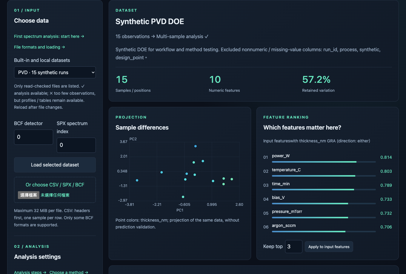
PVD demo: 15 synthetic runs. The projection shows sample differences; the ranking compares process inputs with the selected target.

All demo inputs and results are in data/demo/. Open the demo data browser to choose files and find the matching workbench actions.

For a live artwork demonstration, open Application lab → Artwork differences. Run with seed 7, PCA, 3 components, quantile 0.95 and strength 0.6. Compare the error map with the 18 simulated changed positions. Raise quantile to 0.99 and rerun; then restore 0.95 and lower strength to 0.2. Keep the seed fixed and download each result JSON. The in-app manual includes these steps.

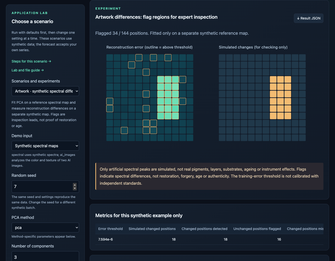
This example uses synthetic spectral maps, not artwork photographs. Real paired-map upload is not available in this lab. A flagged region is a lead for examination, not evidence of retouching or authenticity.

AI silk-painting images — In Application lab → Artwork, choose AI silk-painting images and run the defaults. This reads the two bundled PNGs through patch features → Grey windows → GreyPCA. Hide/show the overlay, then raise quantile to 0.99 and rerun.

Images, computed CSV / JSON and case sources · python3 run.py artwork

Open the interactive review and experiment results — The paired-image view ranks corresponding feature changes for human inspection. The spectral view compares six methods with separate normal calibration and held-out simulation. An identical-PNG control shows why legacy reconstruction flags are not change counts. The region cards demonstrate observations, alternative explanations and next examinations; they are not an expert endorsement.

More demos

Try delivery routes, driver assignment, artwork spectral differences, order forecasting, 2D–4D trajectories, spectroscopy, and semiconductor tools. The image tab also compares AI-generated or uploaded handwriting images.

Read the illustrated walkthrough · PVD CSV · CVD CSV

Note

These examples use synthetic data. They demonstrate the workflow, not production, chemical, or forensic accuracy. Route search and assignment use dedicated optimizers; Grey supplies preference scores. Image distances do not identify writers, and artwork anomalies are investigation leads.

Stability and optimization

GUI walkthrough

Quick entry point: analyze_features() combines ranking stability, GreyPCA regression search and optional normal-data calibration. choose_options() compares named multi-objective alternatives.

import numpy as np
from greytheory import analyze_features

features = np.random.default_rng(7).normal(size=(120, 4))
target = 2 * features[:60, 0] - features[:60, 1]
result = analyze_features(features[:60], target, normal_data=features[60:90])
predictions = result.predict(features[90:])

Quick functions

Check GRA ranking stability, calibrate difference thresholds on separate normal data, search GreyPCA regression settings, and keep Pareto trade-offs among candidate designs.

python3 run.py optimize

Four-step Python guide. The synthetic example needs a repository checkout. Search uses finite random trials and fold-local caching; validation scores are tuning results, not independent test accuracy. Pareto results apply to supplied candidates.

Research models

Experimental equal-step forecasting and quality regression: RL-FGM core, GINN/FGINN engineering variants and independently designed Grey–Fuzzy GPR.

from greytheory import forecast_series

values = [20, 21, 22, 23, 24, 25, 26, 27, 28, 29, 30, 31]
future = forecast_series(values, steps=3, method="rlfgm")
print(future)

GreyPCA + research models

All four models can use pca, sparse, kernel, robust, robust_sparse or adv. Forecast input is a time-by-channel matrix; output restores the original columns. For GINN/FGINN, change method. Backend options go in pca_params={"method_params": {...}}.

import numpy as np
from greytheory import forecast_series, predict_quality

time = np.arange(24.)
history = np.column_stack([20 + time + np.sin(time), 40 + 0.3*time + np.cos(time)])
future = forecast_series(history, steps=3, method="rlfgm",
                         pca_method="adv", n_components=2, order=1)

random = np.random.default_rng(7)
features = random.normal(size=(60, 4))
quality = 100 + 5*features[:, 0] + 2*features[:, 1]**2
result = predict_quality(features[:40], quality[:40], features[40:],
                         pca_method="pca", n_components=2)
print(future, result["prediction"])

In Workbench, choose Research models → Use PCA: on. Forecast components need a declared training-only positive shift; this affects grey models. Quality reliability applies only to retained components.

python3 run.py research

Methods, differences and measured limitations

Documentation

Guide	Contents
Read the illustrated walkthrough	Installation, previews, live analysis, and result files
GreyPCA	All six PCA backends, parameters, and component selection
Images / trajectories	Loading images, feature extraction, and comparison
Bruker	SPX / BCF support and detector calibration
Usage guide	Forecasting, GRA, quality scores, batch jobs, and references

Development

python -m pip install -e . -r requirements-dev.txt
python -m pytest -q
python -m build

Benchmarks · Issues

License

MIT · Third-party notices

Unofficial implementations and rights notices

Algorithms developed with reference to papers in GreyTheory are unofficial implementations, with no affiliation with or endorsement by the original authors or their institutions. Credit for the cited research and its algorithmic contributions belongs to the original researchers.

If you believe an implementation affects your patent, copyright or other rights, please email ilovekalvar@gmail.com with the basis of your concern and the affected algorithm or files. For patent concerns, include the patent number and relevant claims.

We will review notices and, where necessary, correct attribution, modify, suspend or withdraw the relevant algorithms. Receiving a notice or taking precautionary action is not an admission of infringement. Open-source work should respect the contributions of the authors whose research it references.

References

Core Grey and PCA papers

Core references for Grey modelling, PCA, and the implemented robust solvers. Spectral and process-analysis references are in the usage guide.

1. Deng, J. L. (1982). Control problems of grey systems. Systems & Control Letters, 1(5), 288–294.
2. Liu, S. & Lin, Y. (2011). Grey Systems: Theory and Applications. Springer. Grey modelling and relational analysis.
3. Kayacan, E., Ulutas, B. & Kaynak, O. (2010). Grey system theory-based models in time series prediction. Expert Systems with Applications, 37(2), 1784–1789.
4. Jolliffe, I. T. & Cadima, J. (2016). Principal component analysis: a review and recent developments. Philosophical Transactions A, 374, 20150202.
5. Candès, E. J., Li, X., Ma, Y. & Wright, J. (2011). Robust Principal Component Analysis?. Journal of the ACM, 58(3), Article 11. Principal Component Pursuit.
6. Lin, Z., Chen, M. & Ma, Y. (2010). The Augmented Lagrange Multiplier Method for Exact Recovery of Corrupted Low-Rank Matrices. Inexact ALM solver for PCP.
7. Erichson, N. B. et al. (2020). Sparse Principal Component Analysis via Variable Projection, author manuscript. SIAM Journal on Applied Mathematics, 80(2), 977–1002. Robust sparse model: equation (17), Algorithm 2.
8. Vävinggren, D. et al. (2026). A Robust Optimization Approach to Sparse Principal Component Analysis. AdvPCA: Algorithms 1–2 and Appendix A.3.

Research-model sources and implementation attribution

The papers below provide the model definitions and ideas credited to their authors. GreyTheory’s PCA composition, fixed component offsets and quick functions are project integration work; they are not presented as methods proposed by these papers.

• Xu, Zhenguo; Peng, Rui; Pang, Mengyi; Jiang, Jianming; Zhang, Rujing; & Liu, Caixia (2026). A novel grey system model with discrete Riemann–Liouville fractional derivative and its applications. Science Progress, 109(3). Source of the RL-FGM accumulation and response core. GreyTheory uses grid search with a training-tail validation score instead of the paper’s PSO/MAPE selection.
• Xie, Wanli; Zhao, Ruibin; Xu, Zhenguo; & Liang, Tingting (2025). Grey-informed neural network for time-series forecasting. Neurocomputing, 649, 130756. Public preprint, v2 (2024). Source of GINN and FGINN. GreyTheory consulted the public preprint and implements engineering variants with a different network, optimizer and prediction-to-teacher loss; it does not reproduce the authors’ experiments.
• Lawal, Ahmad; Yang, Yingjie; Baisa, Nathanael L.; & He, Hongmei (2026). Reservoir permeability prediction using Integrated Grey-Fuzzy Gaussian Process Regression: A comprehensive framework for uncertainty quantification and interpretability. Engineering Applications of Artificial Intelligence, 177, 114777. Conceptual inspiration for combining GRA, GPR and fuzzy reliability. GreyTheory’s kernel weights and membership rules are independently designed, not a reproduction of the authors’ IGF-GPR.